Take-home_Ex03

Author

YIN HANG

Published

February 14, 2023

Modified

March 11, 2023

In this take-home exercise, we will look into the patterns of the resale prices of public housing property by residential towns and estates in Singapore.

1. R Preparation

Install and launching R packages

The code chunk below uses p_load() of pacman package to check if the necessary packages are installed. If they are, they will be launched into R.

pacman::p_load(tidyverse, dplyr, ggplot2,ggstatsplot, performance, plotly, crosstalk, DT, ggdist, gganimate,FunnelPlotR, knitr)

Importing the data

The code chunk below uses read_csv function to reads the CSV file into a data frame named property_data.

The dataset: Resale flat princes based on registration date from Jan-2017 onwards.

Data is from Data.gov.sg.

property_data <- read_csv("data/resale-flat-prices-based-on-registration-date-from-jan-2017-onwards.csv")

Data Exploration and Analytical Visualisation Selection

Firstly, we will need to understand the data attributes in the selected data set:

Data Attributes	Data Type
month	datetime
town	text
flat type	text
block	text
street name	text
storey range	text
floor area sqm	numeric
flat model	text
lease commence date	datetime
remaining lease	text
resale price	numeric

We can also run summary() to get a glance of the data set.

summary(property_data)

    month               town            flat_type            block          
 Length:146429      Length:146429      Length:146429      Length:146429     
 Class :character   Class :character   Class :character   Class :character  
 Mode  :character   Mode  :character   Mode  :character   Mode  :character  
                                                                            
                                                                            
                                                                            
 street_name        storey_range       floor_area_sqm    flat_model       
 Length:146429      Length:146429      Min.   : 31.00   Length:146429     
 Class :character   Class :character   1st Qu.: 82.00   Class :character  
 Mode  :character   Mode  :character   Median : 94.00   Mode  :character  
                                       Mean   : 97.61                     
                                       3rd Qu.:113.00                     
                                       Max.   :249.00                     
 lease_commence_date remaining_lease     resale_price    
 Min.   :1966        Length:146429      Min.   : 140000  
 1st Qu.:1985        Class :character   1st Qu.: 358000  
 Median :1996        Mode  :character   Median : 448000  
 Mean   :1996                           Mean   : 478124  
 3rd Qu.:2007                           3rd Qu.: 565000  
 Max.   :2019                           Max.   :1418000

In this take-home exercise, we will focus on 3, 4, 5 Room HDB in the study period of 2022.

In order to explore the patterns of the resale prices of public housing property by residential towns and estates in Singapore, there are a few possible affecting factors we can analyse, namely: town, flat type, floor area sqm, flat model and lease commence date/ remaining lease.

Hence from the above, some consideration of the visualization analysis are:

Look into the resale price by 2 different flat midels. We choose standard and DBSS in this exercise. We can build a Two-Sample-Mean-Test to do the comparison.
Then we can focus on standard HDB flat model to do a fair comparison on how other factors affect the resale price. We firstly look at Resale price by town as location is one of the most important factor. We will firstly create a bar chart to show average resale price by town. Then we will do an uncertainty of point estimate to understand the reliability and accuracy of the estimates generated.
Then we start to explore resale price by floor area sqm. We use a scatter plot to visualise the pattern distribution first. Then we conduct a significant test of correlation to understand on their correlation relationship.
As there are a few possible affecting factors, namely: town, flat type, floor area sqm and lease commence date/ remaining lease, we will run a multiple regression model with these factors against resale price to see which factor(s) has/ have higher correlation.
Then we look at flat type (3, 4 or 5 Room HDB) and resale price by using box plot
Lastly we build a heatmap

Analytical Visualisation Preparation

Data preparation

We use filter function from dplyr() package to extract rows that satisfy the given criteria.

extracts rows where the first four characters of “month” column are “2022” to make 2022 as the study period
extract “flat_type” column whereby is “3 Room” ,“4 Room” or “5 Room”.
extract “flat_model” column to be “Standard” or “DBSS” HDB.

The resulting filtered data is stored in a new data frame named filtered_data

filtered_data <- property_data %>%
  filter(substr(month, 1, 4) == "2022", flat_type %in% c("3 ROOM", "4 ROOM","5 ROOM"), flat_model %in% c("Standard","DBSS") )

As the flat_type is in text format, we extract numeric part of flat_type column using mutate() in order to use it for chart plotting.

filtered_data <- filtered_data %>% mutate(flat_type_num = str_extract(flat_type, "\\d+"))

Flat Model (Standard VS DBSS) Resale Price Comparison with Two-sample Mean Test

As DBSS flats are built by private developers with each development characterised by unique external features, it is usually a preferred choice for potential buyers. Hence we would like to compare it’s resale price compared to standard HDB via two-sample mean test, and understand roughly how much premium is required for DBSS flat.

In the code chunk below, ggbetweenstats() is used to build a visual for two-sample mean test of resale price by flat model, namely DBSS and Standard.

ggbetweenstats(
  data = filtered_data,
  x = flat_model, 
  y = resale_price,
  type = "np",
  messages = FALSE
)

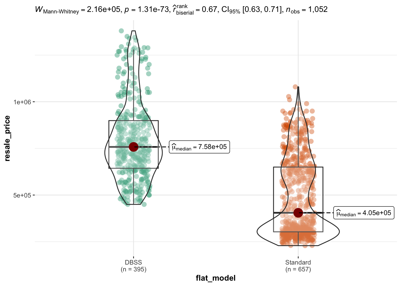
Pattern Observation

We can observe from the above chart, DBSS flat resale price mean is at 758K, compared to that of standard HDB at 405K. There are fewer transactions of DBSS in 2022 (in total 395) compared to standard (in total 657). This could be due to more standard HDB flats in the market.

Resale Price by Town

As now we know that there is a significant difference in resale price between DBSS and Standard HDB, we will narrow down the scope to Standard flat model in order to reduce the number of variables. This will help us to understand the relationship between resale price with other affecting factors, such as town, sqm and flat type better.

Hence, we create another tibble data, standard_data for Standard HDB flat model.

standard_data <- filtered_data %>%
  filter(flat_model == ("Standard") )

Average Resale Price by Town

Use a geom_bar() in ggplot() package to plot a simple bar chart to compare the average resale price of different towns.

Use plotly() to add interactivity to show town name and average resale price of the selected town.

bar_chart <- ggplot(standard_data, aes(x = town, y = resale_price)) +
  geom_bar(stat = "summary", fun = "mean") +
  labs(x = "Town", y = "Average Resale Price") +
  theme(axis.text.x=element_blank(),
        axis.ticks.x=element_blank()) +
  ggtitle("Average Resale Price by Town")

bar_chart <- ggplotly(bar_chart, tooltip = c("town", "resale_price"))

bar_chart

Pattern Observation

From the bar chart, we can observe that the top 3 town based on average resale price are: Bukit Timah, Marine Parade and Clementi. The bottom 3 are: Geylang, Toa Payoh and Kallang/ Whampoa.

Before jumping into conclusion, it is also important to conduct a Uncertainty Test for resale price.

Visualizing the Uncertainty of Point Estimates

We create another tibble data, my_sum, to calculate the mean, standard deviation and standard error of resale price in standard_data.

my_sum <- standard_data %>%
  group_by(town) %>%
  summarise(
    n=n(),
    mean=mean(resale_price),
    sd=sd(resale_price)
    ) %>%
  mutate(se=sd/sqrt(n-1))

Then we use geom_errorbar() function from ggplot() package. We are able to visualise clearly the resale price standard error and the mean resale price indicated by a red dot for different town.

Then convert it to a plotly object using ggplotly() function.

errorbar_plot <- ggplot(my_sum) +
  geom_errorbar(
    aes(x=town, 
        ymin=mean-se, 
        ymax=mean+se)) +
  xlab("town") +
  ylab("resale price standard error with mean") +
  theme(axis.title.x=element_blank(),
        axis.text.x=element_blank(),
        axis.ticks.x=element_blank()) +
    geom_point(aes
           (x=town, 
            y=mean), 
           stat="identity", 
           color="red",
           size = 0.5,
           alpha=1) +
  facet_wrap(~ town) +
  ggtitle("Standard Error of Mean Resale Price by Town")

p_interactive <- ggplotly(errorbar_plot)

p_interactive

Pattern Observation

The above uncertainty of point estimates trellis chart show the range of resale price that the estimate is likely to fall within, with 95% level of confidence.

We can see that the variability in resale price in Clementi is the largest. Whereas in towns such as Bedok, Hougang, Jurong West and Woodlands, there is not much variability in the mean resale price. This will lead to easier price prediction in these regions.

Resale Price by Floor Area in Different Towns

After understanding the differences in average resale prices in various towns, we now add floor area (sqm) into consideration. We look at individual transaction resale price rather than average for this case.

We use geom_point() from ggplot2 package to create a scatter plot to explore the relationship between resale price and floor area, with different colors or shapes representing different towns or estates.

scatter_plot <- ggplot(standard_data, aes(x = floor_area_sqm, y = resale_price, color = town)) +
  geom_point() +
  labs(x = "Floor Area (sqm)", y = "Resale Price", color = "Town") +
  ggtitle("Scatter plot of Resale Price vs. Floor Area by Town")

scatter_plot <- ggplotly(scatter_plot, tooltip = c("town","floor_area_sqm", "resale_price"))

scatter_plot

Pattern Observation

We observe that even though Bukit Timah has the highest average resale price, the top 3 resale price transactions are for HDB in Maria Parade.

The common assumption is the bigger the floor area, the higher the resale price. In order to understand more about the correlation between floor area sqm and resale price, we will run a Significant Test of Correlation.

Significant Test of Correlation

In the code chunk below, ggscatterstats() is used to build a visual for Significant Test of Correlation between floor area (sqm) and resale price (S$).

ggscatterstats(
  data = standard_data,
  x = floor_area_sqm,
  y = resale_price,
  marginal = FALSE,
  )

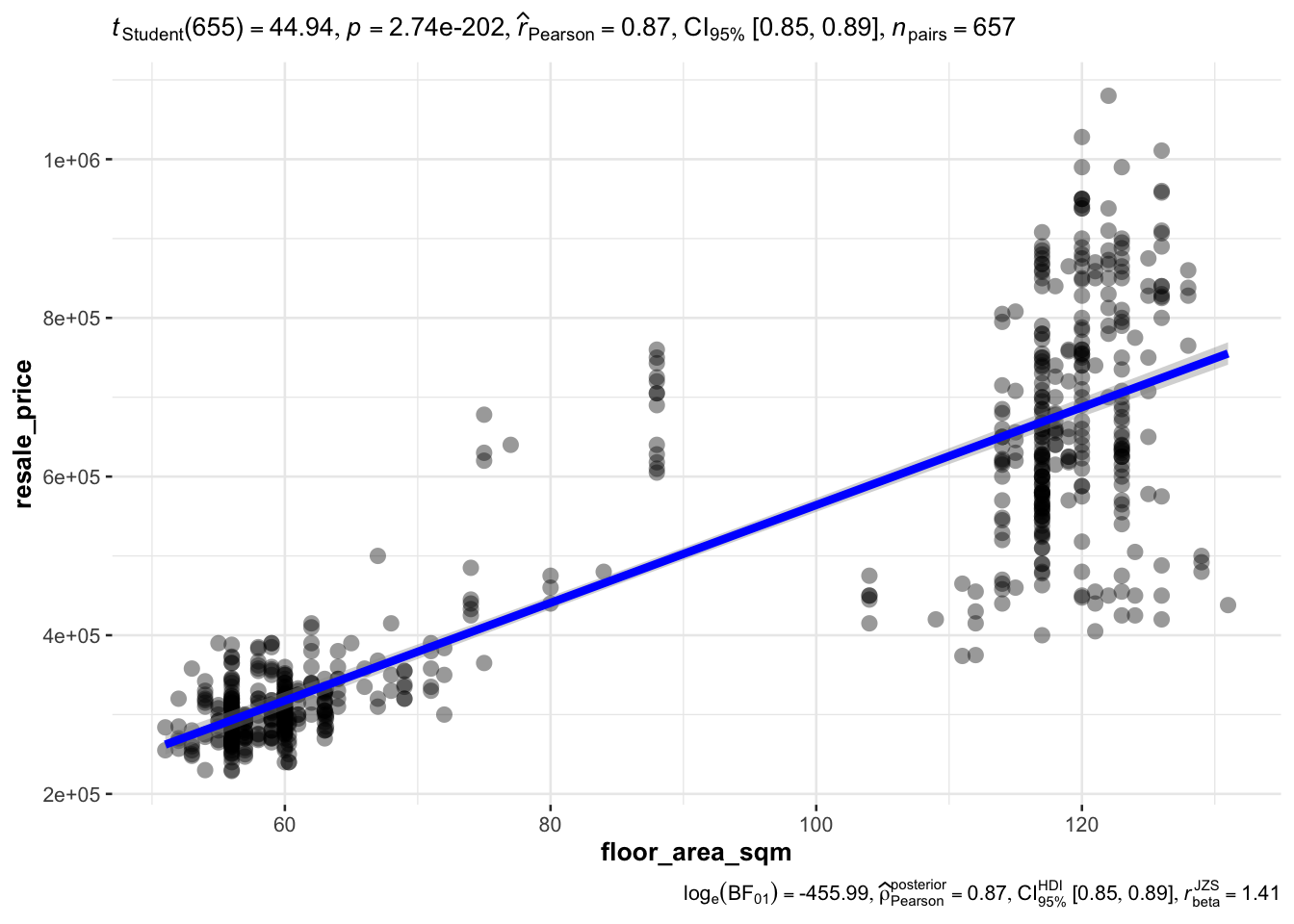
Pattern Observation

From the above t-test with sample size of 657 transactions, we see a linear correlation between floor area (sqm) VS resale price. The correlation coefficient, r(pearson) = 0.87, indicating a positive linear relationship between floor area (sqm) and resale price. The small p value indicates statistic significance.

However, there are still outliers which fall far away from the linear regression line.

Hence we will continue the exploration by looking into Multiple regression model to consider other factors.

Multiple Regression Model

We will add in lease commence date and flat type into the model and build a multiple regression model. This is to analyse how these other factors affecting the resale price besides floor area.

model <- lm(resale_price ~ floor_area_sqm + lease_commence_date + flat_type_num, data = standard_data)

summary(model)


Call:
lm(formula = resale_price ~ floor_area_sqm + lease_commence_date + 
    flat_type_num, data = standard_data)

Residuals:
    Min      1Q  Median      3Q     Max 
-370302  -48060   -5561   45874  367167 

Coefficients:
                     Estimate Std. Error t value Pr(>|t|)    
(Intercept)         5268643.6  3192415.2   1.650   0.0994 .  
floor_area_sqm        11242.0      685.1  16.410  < 2e-16 ***
lease_commence_date   -2854.3     1624.3  -1.757   0.0793 .  
flat_type_num4       -57666.9    35704.0  -1.615   0.1068    
flat_type_num5      -290137.3    40508.0  -7.162 2.15e-12 ***
---
Signif. codes:  0 '***' 0.001 '**' 0.01 '*' 0.05 '.' 0.1 ' ' 1

Residual standard error: 100300 on 652 degrees of freedom
Multiple R-squared:  0.7751,    Adjusted R-squared:  0.7737 
F-statistic: 561.8 on 4 and 652 DF,  p-value: < 2.2e-16

Pattern Observation

From the small p-value, we know that at least one of the factors are affecting the resale price significantly. The R-squared value, 0.7737 shows a generally good fit of the model. But before concluding whether this is a good regression model, we will need to check for multicolinearity.

Model Diagnostic: Checking for Multicolinearity

check_collinearity(model)

# Check for Multicollinearity

Low Correlation

           Term   VIF     VIF 95% CI Increased SE Tolerance Tolerance 95% CI
 floor_area_sqm 27.06 [23.34, 31.40]         5.20      0.04     [0.03, 0.04]

High Correlation

                Term   VIF     VIF 95% CI Increased SE Tolerance
 lease_commence_date  3.00   [2.65, 3.41]         1.73      0.33
       flat_type_num 26.49 [22.85, 30.74]         5.15      0.04
 Tolerance 95% CI
     [0.29, 0.38]
     [0.03, 0.04]

Pattern Observation

From the Multicollinearity check, we know that floor area sqm is a good predictor variable as it has a low correlation. However, the lease commence date and flat type have high correlation. Hence we might need to analyse them separately.

Resale Price Distribution by Flat Type in Different Towns

We use geom_boxplot() under ggplot() package to create a box plot.

This helps in visualising the distribution of resale prices for different flat types and towns.

box_plot <- ggplot(standard_data, aes(x = flat_type, y = resale_price)) +
  geom_boxplot() +
  labs(x = "Flat Type", y = "Resale Price") +
  ggtitle("Resale Price Distribution by Flat Type")

box_plot <- ggplotly(box_plot, tooltip = "resale_price")

box_plot

Pattern Observation

Generally, the average resale price is highest for 5 Room, followed by 4 Room and 3 Room.

There are the most number of outliers for 3 Room flat resale prices, meaning some transaction of 3 Room flat sell at very high prices.

The resale prices for 4 Room flat are closely distributed, the variability is the smallest.

The resale price range for 5 Room flat are the biggest.

Heatmap Visualization on Resale Price, Floor Area sqm and Lease Commence Date

With all the above analysis, now we want to build a heatmap to visualize at a glance.

We use geom_tile() from ggplot() to plot a heatmap to visualize between different variables, such as resale price, floor area, and lease commence date/ year.

heatmap <- ggplot(standard_data, aes(x = factor(lease_commence_date), y = factor(floor_area_sqm), fill = resale_price)) +
  geom_tile() +
  labs(x = "Lease Commence Year", y = "Floor Area (sqm)", fill = "Resale Price") +
  ggtitle("Heatmap of Correlation between Resale Price, Floor Area, and Year")

ggsave("heatmap.png", heatmap, height = 8, units = "in")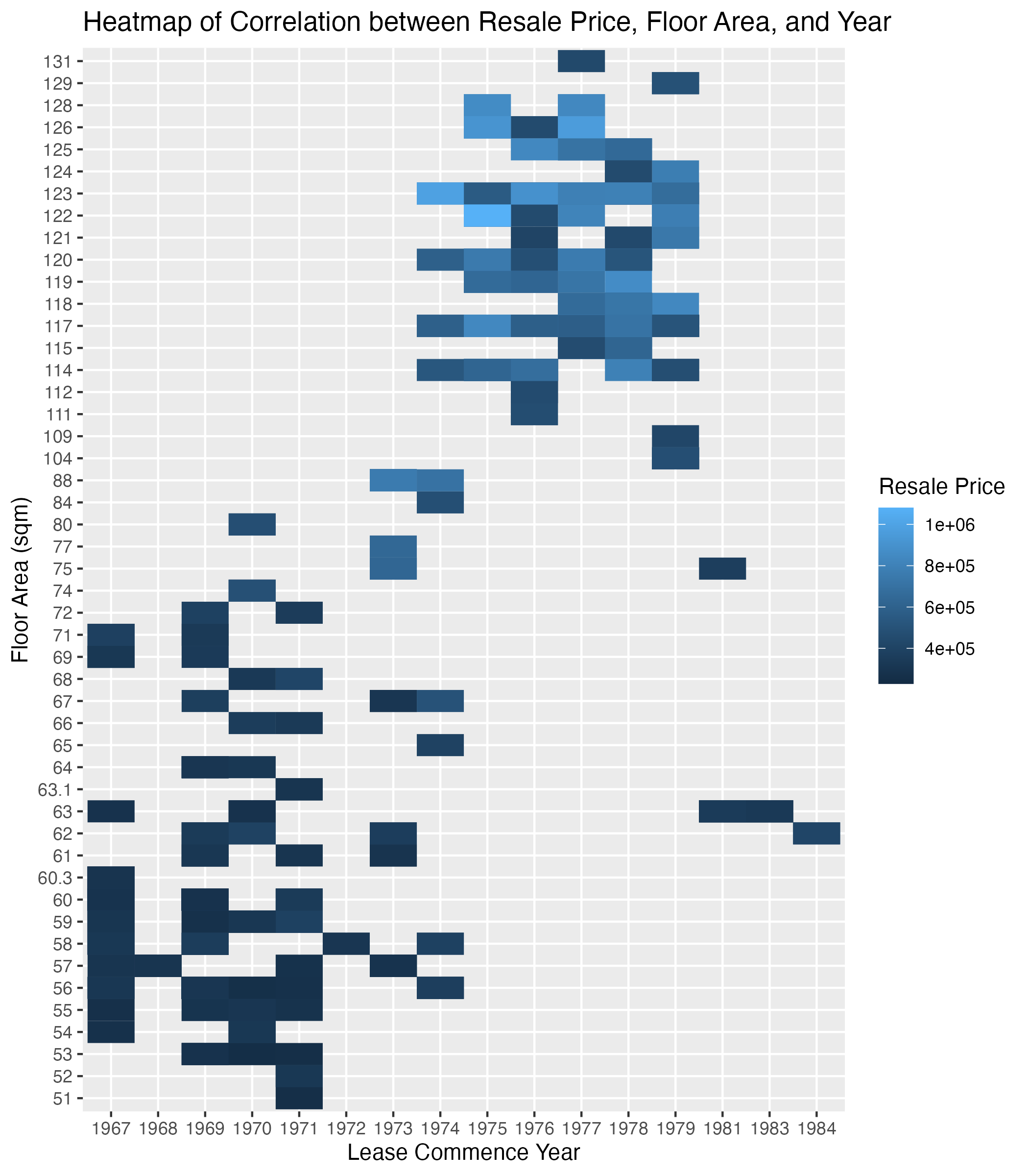

Pattern Observation

We can see when taking lease commence year and floor area, generally the newer the flat (later lease commence year) and bigger the size (bigger floor area), the higher the resale price (lighter in blue color tone). However there are also some outliers.

Hence it is really not enough to look at one aspect of the HDB property to predict the price, all these factors: town, flat type, floor area sqm, flat model and lease commence date/ remaining lease, play a part in influencing the resale price.

The above concludes my Take Home Exercise 3.

Thank you for reading!